
Are you spending too much time scanning spreadsheets to find overdue tasks, duplicate entries, or low-performing sales numbers? Manually highlighting important data is time-consuming, inconsistent, and very easy to miss. Here’s how you can apply Conditional Formatting in Excel so that important information can stand out automatically in just a few clicks.
Apply Conditional Formatting by going to Home → Conditional Formatting, choosing a rule, configuring the required conditions, and clicking OK.
Conditional Formatting automatically changes a cell’s appearance when it meets specific conditions, such as values greater than a number, duplicate entries, dates, or formulas. Instead of manually reviewing every row, Excel instantly highlights the cells that match your criteria, making trends and issues much easier to identify.
If sales below 500 should be highlighted:
Excel automatically highlights values below 500.
What Is Conditional Formatting in Excel?
Conditional Formatting is an Excel feature that automatically changes a cell’s formatting when certain conditions are met. Instead of manually coloring cells every time your data changes, Excel updates the formatting automatically. Examples include:
- Highlight dates that are overdue
- Identify duplicate values
- Show which are top-performing sales
- Visualize trends using color scales
Benefits of Using Conditional Formatting
Using Conditional Formatting helps you by:
- Quickly identify important data
- Reducing manual formatting work
- Improve report readability
- Spot errors instantly
- Create dynamic dashboards
- Monitor KPIs automatically
It’s one of the fastest ways to make large spreadsheets easier to analyze.
How to Apply Conditional Formatting in Excel (Step-by-Step)
Step 1: Select Your Data
- Click and drag to highlight the exact range you want Excel to evaluate.
- Example: C2:C16
Common Mistake: Conditional formatting only applies to the cells you select. Selecting the wrong range causes some cells to remain unformatted.
Step 2: Open the Conditional Formatting Menu
- On the Excel Ribbon, go to:
- Home → Conditional Formatting
- You’ll see several built-in options such as Highlight Cells Rules, Top/Bottom Rules, Data Bars, Color Scales, and Icon Sets.
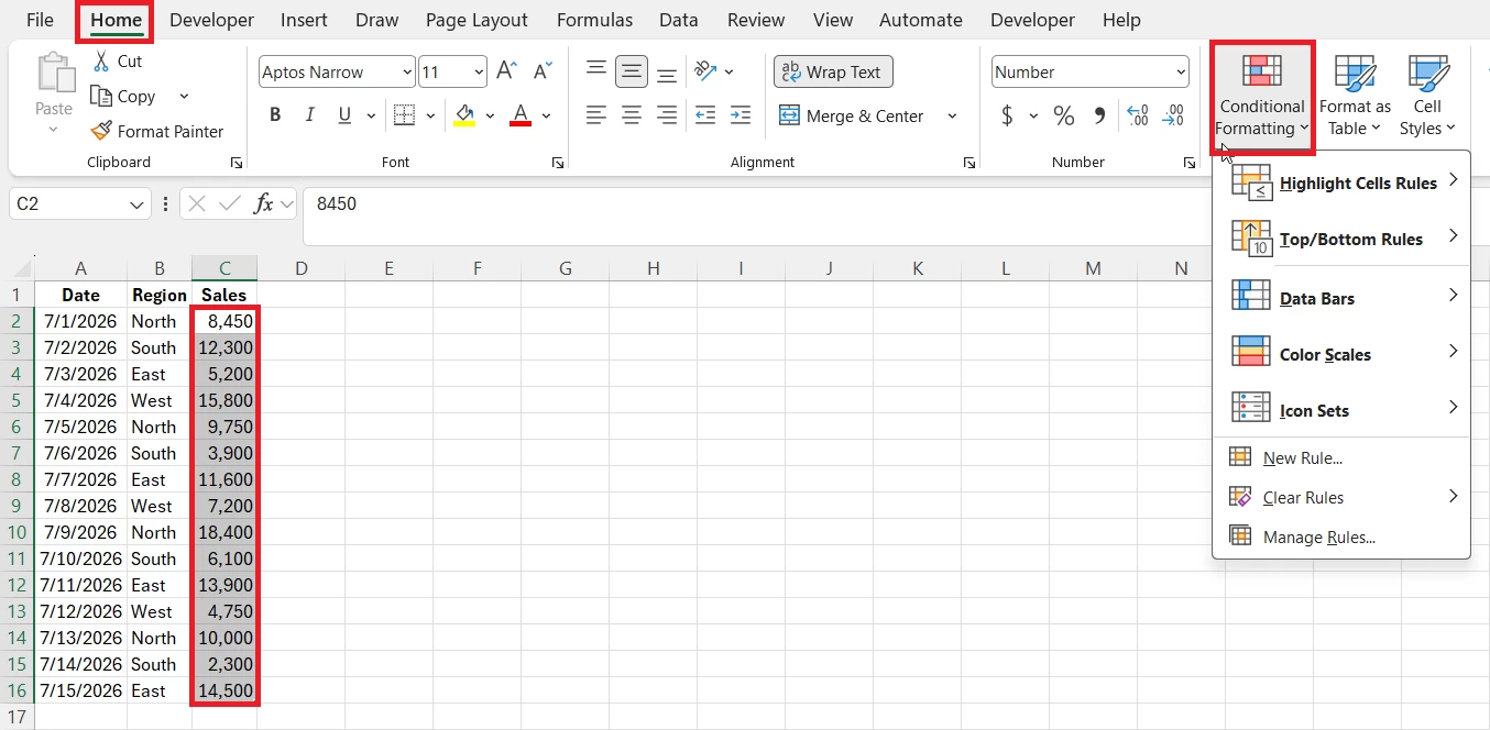
Common Mistake: Clicking Format Cells instead of Conditional Formatting. Format Cells changes appearance manually and won’t update automatically when data changes.
Step 3: Choose a Built-in Rule
Choose a rule that matches the logic you need, for example:
- Greater Than
- Less Than
- Between
- Equal To
- Text that Contains
- A Date Occurring
- Duplicate Values

Each rule type evaluates data differently. Pick the one that matches the condition you want Excel to check.
Common Mistake: Choosing the wrong rule for your goal (e.g., using Text Contains for numbers). Read the rule label before selecting it.
Step 4: Define the Formatting Condition
- Enter the comparison value or expression.
- Example: Highlight numbers that are greater than 9000.
- Enter 9000
- Choose the formatting through with option (fill color, font color, bold, etc.),
- Then click OK.
Common Mistake: Entering text when the rule expects a number. If your data are numbers, make sure the condition is numeric; if dates, use a date format.
Step 5: Review the Results
- Excel immediately highlights every matching value. If the data changes later, formatting updates automatically.
- Edit the rule later if needed: Home → Conditional Formatting → Manage Rules.
Common Mistake: Assuming formatting is static. If you edit values, the highlights will recalculate, so always recheck after major edits or after copying/pasting data.
Types of Conditional Formatting Rules in Excel
Below are Excel’s ready-to-use conditional formatting rule types, what each one does, when to use it, a short example, and a quick tip to avoid mistakes.
Highlight Cells Rules
It checks individual cell values against a simple condition and applies formatting to matches. It is useful for:
- Greater Than
- Less Than
- Between
- Equal To
- Text that Contains
- A Date Occurring
- Duplicate Values
- Example: Highlight all scores below 40.
Top/Bottom Rules
Finds values relative to the rest of the range and highlights extremes or outliers. It is perfect for finding:
- Top 10 values
- Bottom 10 values
- Above Average
- Below Average
- Example: Highlight the top 5 sales representatives.
Data Bars
Creates horizontal bars inside cells to compare values visually. Ideal for:
- Sales comparisons
- Budget tracking
- Performance reports
- Example: Use data bars to show monthly revenue differences across regions.
Color Scales
It applies different colors based on value ranges.
Example:
- Green = High
- Yellow = Medium
- Red = Low
Icon Sets
Places icons next to values to show categories or trends.
- Arrows
- Traffic lights
- Stars
- Flags
- Example: Green or up arrow for displaying improving metrics, red down arrow for declines. It is great for KPI dashboards.
How to Create a Custom Conditional Formatting Rule
Use a formula when built‑in rules can’t express the logic you need. A formula rule evaluates each cell in the selected range and applies formatting when the formula returns TRUE. Formula rules are powerful because they can reference other columns, test multiple conditions, and format entire rows.
Example: Highlight an entire row when Sales in column C exceed 5,000. Using the formula below:
=$C2>5000This formula checks the value in column C for each row; if it’s greater than 5,000, the formatting is applied to every cell in that row inside the selected range.
Steps to Create a Custom Conditional Formatting Rule:
- Select the entire table.
- Go to Home → Conditional Formatting → Select New Rule.
- Choose Use a formula to determine which cells to format.
- Type =$C2>5000 into the formula box.
- Click Format, pick fill color, font, or border, then click OK.
- Click OK againto create the rule and check the sheet for expected highlights.
Understanding How the Formula Works
- The leading equals sign tells Excel this is a formula.
- $C locks the column, so the rule always checks column C as Excel evaluates each cell across the row.
- Row reference (2) is relative, so Excel adjusts it for each row (2 becomes 3, 4, 5, etc.).
- If the formula returns TRUE for a row, Excel applies the chosen formatting to every cell in the selected range for that row.
Common Mistake: Forgetting to lock the correct column with the $ symbol, locking the row instead of the column, selecting the wrong range, or Mismatched data types.
How to Edit, Copy, Clear, and Manage Conditional Formatting
Use the Manage Rules dialog to review, change, and control how conditional formatting behaves across your workbook. This central tool lets you edit conditions, remove rules, change which cells they apply to, and set rule precedence to ensure predictable results.
To edit existing rules:
- Go to Home → Conditional Formatting → Manage Rules.
- In the dialog, set Show formatting rules for to This Worksheet or Current Selection depending on the scope you want to edit.
- Select the rule you want to change and click Edit Rule
Edit an Existing Rule
- Change condition: Update the built‑in options or the formula that returns TRUE/FALSE.
- Adjust the format: Click Format to change fill, font, border, or number formatting.
- Change the range: Edit the Applies to field to expand or restrict which cells the rule covers.
- Click OK to save each change, then Apply or OK to close the dialog.
You can also Delete, Pause, or Reapply Rules:
- Delete a rule by selecting it and clicking Delete Rule.
- Stop If True: Enable this option to prevent lower‑priority rules from running when the current rule matches.
- Reapply rules after major edits or after copying and pasting data by using Home → Conditional Formatting → Clear Rules and then reapplying, or by using Manage Rules to adjust ranges.
Change Rule Priority
- Use Move Up and Move Down inside Manage Rules to reorder rules.
- The rule at the top has the highest priority when rules conflict.
- Review the preview column to see which format will appear when multiple rules apply.
Common Mistake: Editing only the active worksheet instead of “This Worksheet“, forgetting to update the Applies To range after copying rows, Conflicting rules with wrong priority, or accidentally editing the wrong rule.
Conditional Formatting Keyboard Shortcuts
Excel doesn’t have a dedicated keyboard shortcut that opens Conditional Formatting directly. Some of the useful shortcuts include:
| Shortcut | Action |
| Alt + H + L | Open Conditional Formatting menu |
| Alt + H + L + H | Highlight Cells Rules |
| Alt + H + L + T | Top/Bottom Rules |
| Alt + H + L + D | Data Bars |
| Alt + H + L + S | Color Scales |
| Alt + H + L + I | Icon Sets |
These shortcuts help you navigate the Conditional Formatting menu without using the mouse.
Common Conditional Formatting Mistakes (and How to Fix Them)
Conditional formatting is powerful but easy to misapply. Below are the five most frequent mistakes, why they cause problems, and precise fixes you can apply immediately.
1. Selecting the Wrong Range
Conditional formatting only evaluates the cells you select. If the selection is too small or offset, some rows or columns will never be formatted. Always verify the selected cells before creating a rule.
- What to check: Look at the Name Box or the Applies to field in Manage Rules to confirm the exact range.
- How to Fix: Select the full table or the exact rows/columns you want before creating the rule; update Applies to afterward if you add rows.
2. Using Incorrect Cell References in Formulas
Wrong absolute and relative references make Excel test the wrong cells, producing inconsistent or no formatting. Incorrect absolute ($) and relative references often produce unexpected results.
- What to check: Open Manage Rules and inspect the formula for $ placement and the starting row number.
- How to Fix Use $ to lock columns you always want referenced (for example, =$C2>5000) and leave the row relative so it adjusts per row.
3. Creating Too Many Rules
Multiple overlapping or redundant rules slow workbook performance and make results hard to interpret.
- What to check: In Manage Rules, count rules that apply to the same range and look for duplicates or near‑duplicates.
- How to Fix: Consolidate similar rules into one formula rule or use icon sets/color scales instead of many single‑value rules.
4. Ignoring Rule Order and Priority
When multiple rules apply, Excel evaluates them in order; the top rule can override others.
- What to check: Open Manage Rules and review the order; check whether Stop If True is enabled for any rule.
- How to Fix: Reorder rules with Move Up/Move Down and use Stop If True to prevent lower rules from applying when a higher rule matches.
5. Forgetting Dynamic Updates
Conditional formatting recalculates automatically; manually recoloring cells breaks the rule logic and creates inconsistencies.
- What to check: Change a sample value in the range and see whether formatting updates. If it doesn’t, the rule may not cover that cell.
- How to Fix: Avoid manual coloring inside formatted ranges; extend the rule range or convert the range to an Excel Table so rules auto‑expand.
Real-World Examples of Conditional Formatting
Use conditional formatting to surface issues and insights automatically so you spend less time scanning spreadsheets and more time acting on results. Where you’ll use this:
Sales Dashboard
- Automatically highlight sales above target, below quota, or the top-performing products to make monthly reports easier to review.
- Example rule: Highlightsales greater than target: Cell Value > Target, or use a formula to compare each row to a target column.
Project Management
- Flag overdue deadlines, completed tasks, or upcoming milestones without manually updating cell colors.
- Example rule: Highlight overdue tasks: Due Date <TODAY() with a red fill; highlight completed tasks by checking a Status column equals “Done”.
Finance & Budgeting
- Identify overspending, negative balances, or unusually high expenses so issues stand out immediately.
- Example rule: Highlight negative balances: Cell Value < 0 in the Balance column; highlight expenses above a threshold with a color scale or icon set.
Key Takeaway
- Conditional Formatting automatically highlights important data based on rules, saving time and reducing manual work.
- Built-in rules cover most everyday needs, while formula-based rules offer advanced customization for dynamic reports.
- Use keyboard shortcuts like Alt + H + L and regularly review rule priority through Manage Rules to keep formatting accurate and efficient.