
You’ve built a clean SUM formula. Then one #N/A error appears in your range, and the entire total collapses into an error message. Manually hunting down and deleting each #N/A isn’t just tedious; it defeats the purpose of having a dynamic spreadsheet.
The good news is that Excel gives you several ways to SUM in Excel while ignoring #N/A errors. The trick is choosing the right formula for your specific situation. Do you need to ignore only #N/A, or should every error type be excluded? The answer changes which formula you should use. This guide gives you working formulas, then explains when to use each one so you can pick the right approach.
Ignore all errors:
=AGGREGATE(9,6,A2:A20)
Returns the sum of numeric values while ignoring
#N/A, #DIV/0!, #VALUE!,
and other errors.
Ignore only #N/A:
=SUM(IFNA(A2:A20,0))
Treats #N/A as 0 while leaving other errors visible.
| Need | Formula |
|---|---|
| Ignore all errors | =AGGREGATE(9,6,range) |
| Ignore only #N/A | =SUM(IFNA(range,0)) |
| Ignore all errors with IFERROR | =SUM(IFERROR(range,0)) |
| Fix lookup-generated #N/A | Use IFNA in the source formula |
A2:A5 contains 100, 250, #N/A, and 50, =AGGREGATE(9,6,A2:A5) returns 400.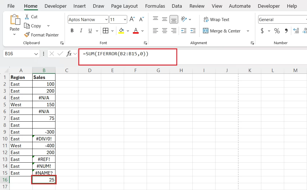
Why Does SUM Return #N/A in Excel?
When you reference a range that contains an error value, SUM can’t complete its calculation. The error isn’t just a display issue it’s a value that SUM cannot process as a number.
Example Data:

Formula:
=SUM(A2:A5)The #N/A in the range propagates through the entire calculation. Excel can’t add a number to an error, so the whole formula returns that error. This is why you need a formula that specifically handles or excludes error values before the SUM operation completes.
How to SUM in Excel While Ignoring #N/A Step-by-Step
Step 1: Identify Where Your Data Lives
- Open the workbook and locate the column or range containing values you want to sum.
- What you should see: A column of numbers with one or more
#N/Aerrors mixed in.
Common Mistake: Accidentally selecting the header row in your range. If A1 contains “Sales” and your data starts at A2, use A2:A20, not A1:A20.
Step 2: Choose a Formula Based on the Error Type
Ask yourself, “Do I only need to ignore #N/A, or should I ignore every error type?”
- For
#N/Ause the below formula:
=SUM(IFNA(A2:A5,0))- For all other errors use:
=AGGREGATE(9,6,A2:A20)- What you should see: Your formula in the formula bar, with the range matching your actual data.
Common Mistake: Using IFERROR when you only want to ignore #N/A. This hides other errors that might indicate real problems.
Step 3: Enter the Formula and Verify the Result
Type your chosen formula into an empty cell and press Enter.
What you should seenow is a numeric result, not an error message. The total should match what you’d get if you manually added only the valid numbers.
Common Mistake: Not testing with a known dataset first. Always verify your formula works with sample data before applying it to critical reports.
Step 4: Test the Formula with Edge Cases
Add a temporary #DIV/0! or #VALUE! error to your range to confirm your formula behaves as expected.
What you should see:
AGGREGATE(9,6,...)ignores all error typesSUM(IFNA(...))ignores only#N/A; other errors still break the formula
Common Mistake: Assuming all “ignore error” formulas work the same way. They don’t.
4 Methods to SUM in Excel While Ignoring #N/A
Method 1 — Use AGGREGATE to Ignore Errors
Formula to SUM While Ignoring Errors:
=AGGREGATE(9,6,B2:B12)How AGGREGATE Ignores #N/A Values
| Component | Meaning |
| 9 | Function number for SUM |
| 6 | Option to ignore error values |
| B2:B12 | Your data range |
AGGREGATE is designed to perform calculations while optionally ignoring errors, hidden rows, or both. The second argument (6) specifically tells it to skip error values.
When to Use AGGREGATE
- Your range contains
#N/A - Your range may contain other Excel errors (
#DIV/0!, #VALUE!,etc.) - You want to sum numeric values while ignoring all error values
Important Limitation of AGGREGATE
AGGREGATE ignores error values but does not ignore:
- Blank cells (they contribute nothing)
- Text values (they’re ignored in
SUMoperations) - Negative numbers (these are included)
Tested Behavior:
| Data Type | AGGREGATE Behavior |
#N/A | Ignored |
#DIV/0! | Ignored |
#VALUE! | Ignored |
| Blank cells | Ignored (no effect) |
| Text | Ignored (no effect) |
| Positive numbers | Included |
| Negative numbers | Included |
Method 2 — Use IFNA to Ignore Only #N/A Values
Formula to SUM and Ignore #N/A:
=SUM(IFNA(A2:A7,0))How IFNA Works
IFNAevaluates each cell in the range. If a cell contains#N/A,IFNAreplaces it with0.- All other values, including other error types, pass through unchanged.
Example: SUM with IFNA:
=SUM(IFNA(A2:A7,0))returns375- The two
#N/Avalues become0. The remaining numbers(100 + 250 - 50 + 75)sumto375.
Why IFNA Can Be Better Than IFERROR
=IFNA(...)targets only#N/Aerrors.=IFERROR(...)handles all Excel error types.
This distinction matters. An unexpected #DIV/0! or #VALUE! might indicate a real problem in your data: a broken formula, a missing reference, or incorrect input. IFNA lets those errors surface so you can investigate, while still handling the expected #N/A from lookups.
Method 3 — Use IFERROR When All Errors Should Be Ignored
Formula to SUM While Ignoring All Errors:
=SUM(IFERROR(B2:B15,0))How IFERROR Works
IFERRORconverts any error value to zero. This includes#N/A,#DIV/0!,#VALUE!,#REF!,#NAME?,#NUM!, and#NULL!.- Use this when your business logic says any error should contribute nothing to the total.
IFNA vs IFERROR
| Formula | Handles #N/A | Handles Other Errors |
IFNA | Yes | No |
IFERROR | Yes | Yes |
Note: Suppressing every error can hide problems in your underlying data. If you use IFERROR, make sure you’re not masking issues that need attention. A #DIV/0! might mean a denominator is zero. A #VALUE! might mean text is where a number should be. These aren’t always safe to ignore.
Method 4 — Use SUMIF to Exclude #N/A Values
Formula to Exclude #N/A from a SUM:
=SUMIF(B2:B10,"<>#N/A")How SUMIF Works
- The criterion “
<>#N/A” tellsSUMIFto sum only cells that are not equal to#N/A. - Limitation:
SUMIFwith this criterion excludes#N/Abut does not handle other error types.
Tested Behavior:
| Data Type | SUMIF Behavior |
#N/A | Excluded |
#DIV/0! | Returns error |
#VALUE! | Returns error |
| Negative numbers | Included |
| Text | Ignored |
If your range contains #DIV/0! or #VALUE!, SUMIF will return an error. This makes SUMIF less robust than AGGREGATE or IFERROR for general error handling.
When to Use SUMIF
- You’re certain the only error type is
#N/A - You need conditional summing (e.g., sum by category)
- You want a simple, readable formula
How to SUM Only Numeric Values Without Losing Negative Numbers
A common shortcut is:
=SUMIF(A2:A6,">0")This sums only positive numbers. It appears to “work” because it skips errors which aren’t greater than zero. But it also excludes negative numbers, which are often valid data.
Example: SUM Numeric Values While Ignoring #N/A:
=SUMIF(A2:A6,">0")returns425(excludes -50)=SUM(IFNA(A2:A6,0))returns375(includes -50)- The correct error-handling solution should include
-50. - A
>0criterion incorrectly excludes it.
Note: Never use >0 as an error-handling shortcut. Use IFNA, IFERROR, or AGGREGATE instead.
How to Use SUMIFS When the Range Contains #N/A
SUMIFS adds complexity because you’re filtering by criteria while also dealing with errors in the sum range.
Example Use Case: Sum sales for the East region while ignoring unavailable values.
Problem: =SUMIFS(B2:B7, A2:A7, "East") returns #N/A because the sum range contains errors.
Workaround: Wrap the sum range in IFERROR or use AGGREGATE with a conditional approach.
Tested Formula:
=SUM(IFERROR(SUMIFS(B2:B7,A2:A7,"East"),0))However, this returns 0 if any error exists, not the sum of valid East values.
A better approachis to fix the source data or use a helper column that converts errors to zero, then SUMIFS on that column.
Limitation: SUMIFS does not natively ignore errors in the sum range. You must pre-process the data or use array formulas.
What If the #N/A Comes from a Lookup Formula?
Sometimes the best solution isn’t fixing the SUM formula; it’s fixing the source.
#N/A often originates from:
XLOOKUPVLOOKUPINDEX/MATCHMATCH- Other lookup or calculation formulas
Source-Level Fix for #N/A:
=IFNA(XLOOKUP(...),0)This handles the error where it occurs, making downstream calculations simpler.
Important Distinction
- Use zero only if “not found” should logically contribute zero
- Do not convert a meaningful missing-data condition into zero simply to make the
SUMwork - If a missing value indicates a data problem, masking it with zero could lead to incorrect totals and bad decisions.
Which Formula Should You Use to Ignore #N/A in Excel?
| Your Situation | Use |
Only #N/A should be ignored | SUM(IFNA(range,0)) |
| Any error should be ignored | AGGREGATE(9,6,range) |
| Any error should become zero | SUM(IFERROR(range,0)) |
| Need a conditional sum | SUMIF / SUMIFS |
| Error originates from a lookup | Consider fixing the lookup |
| Negative numbers are valid | Avoid >0 shortcuts |
Common Mistakes When Ignoring #N/A in Excel
Mistake 1: Using Normal SUM
=SUM(A2:A20)This formula fails when the range contains #N/A. You need a formula that handles errors.
Mistake 2: Using IFERROR When Only #N/A Should Be Handled
IFERRORhides all errors. If a#DIV/0!appears due to a broken formula, you won’t see it.- Use
IFNAwhen you specifically want to ignore only#N/A.
Mistake 3: Using >0 to Bypass Errors
This excludes negative numbers, which are often valid. Use IFNA, IFERROR, or AGGREGATE instead.
Mistake 4: Assuming Every Formula Handles Every Error
#N/Ais different from#DIV/0!,#VALUE!, and other errors.IFNAhandles only#N/A.SUMIFwith “<>#N/A” handles only#N/A. Know the difference.
Mistake 5: Hiding a Problem Instead of Fixing Its Source
If #N/A comes from a lookup that can’t find a match, consider whether the lookup itself should be fixed. Sometimes the best solution is =IFNA(XLOOKUP(...),0) at the source.
Excel Version Considerations
| Formula | Microsoft 365 | Excel 2021 | Excel 2019 | Older Versions |
AGGREGATE | Yes | Yes | Yes | Excel 2010+ |
IFNA | Yes | Yes | Yes | Excel 2013+ |
IFERROR | Yes | Yes | Yes | Excel 2007+ |
SUMIF | Yes | Yes | Yes | All versions |
Note: In older Excel versions, =SUM(IFNA(A2:A20,0)) may require Ctrl+Shift+Enter to work as an array formula. In Microsoft 365 and Excel 2021, it works as a normal formula due to dynamic arrays.
Real Use Cases
- Financial Reports: Monthly sales data pulled from multiple sources often contains
#N/Afrom failed lookups. You need totals that reflect actual numbers, not error messages. - Inventory Tracking: Product codes that don’t match between systems create
#N/Aerrors. Summing quantities while ignoring those errors keeps your stock calculations accurate. - Survey Analysis: Exported data often contains
#N/Afor skipped questions. Summing response scores while ignoring non-responses gives you valid totals. - Budget vs. Actuals: When actual figures haven’t been entered yet, lookups return
#N/A. Your variance calculations need to handle this gracefully.
Key Takeaway
- Normal
SUMdoes not ignore error values. You need a formula that specifically handles errors before summing. - Use
IFNAwhen only#N/Ashould be ignored. UseAGGREGATEwhen error values generally should be ignored. UseIFERRORwhen all errors should intentionally become zero. - Fix the source formula instead when that’s the better data-handling decision. Sometimes the right answer isn’t a better
SUM; it’s a better lookup.