
Have you ever lost track of your headers while scrolling through endless rows of data? Scrolling through large Excel worksheets can be a headache, especially when your headers or key labels disappear. Freezing cells in Excel helps you keep your view organized, no matter how large your spreadsheet becomes. In this guide, I’ll walk you through everything from freezing the top row and first column to customfreeze options, plus how to remove freezes when needed. You’ll also learn the key differences between Freeze Panes vs Split Panes, and when to use each for maximum efficiency.
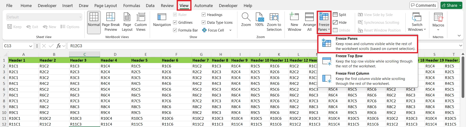
To freeze cells, rows, or columns in Excel, go to View → Freeze Panes.
Choose Freeze Top Row, Freeze First Column, or Freeze Panes depending on what you want to keep visible while scrolling.
- Freeze Top Row — Keeps the first row visible while you scroll down.
- Freeze First Column — Keeps the first column visible while you scroll horizontally.
- Freeze Panes — Freezes all rows above and columns to the left of the selected cell.
If you select C3 and choose
View → Freeze Panes → Freeze Panes, Excel will freeze:
- Rows 1 and 2
- Columns A and B
The frozen rows and columns remain visible while you scroll through the rest of the worksheet.
You can keep headings, labels, or other important information on screen while working with large Excel spreadsheets.
What is Freeze Panes in Excel
Freeze cells in Excel means locking the specific rows or columns in place so that they stay visible while you scroll through the rest of the worksheet. In Excel this feature is called Freeze Panes.
What Freeze Cells actually does
- When you freeze a row, that row will stay fixed at the top of the worksheet while you scroll down.
- When you freeze a column, that column stays fixed at the left while you scroll right and,
- When you freeze panes at a particular cell, Excel keeps everything above that cell and to the left of that cell visible while the rest of the sheet scrolls.
Example
If you’re working with employee data that includes headers like Manager Name, Senior Manager Name, Department Name, Band, etc., you’ll notice that as you scroll down, the headers disappear from view. This is where the Freeze Panes feature becomes incredibly useful, it allows you to keep those important headers visible at all times while navigating through your data, so that you know which data belongs to which particular category.
How to Freeze Panes in Excel
Freeze the Top Row in Excel

- In the Excel Ribbon, go to the View tab.
- Click on the Freeze Panes.
- Select Freeze Top Row.
- Freeze Top Row option keeps the first row visible when scrolling down in the worksheet.
Freeze the First Column in Excel
- Go to the View tab.
- Click on Freeze Panes.
- Select Freeze First Column.
- The Freeze First Column option keeps the first column visible when scrolling towards the right.
Freeze Rows and Columns at the Same Time in Excel
If you want to freeze rows and columns at the same time in Excel, you can do this with the Freeze Panes option. This is a very useful feature for large worksheets where you need to keep both your column headings and row labels visible while scrolling. The key here is to select the cell immediately below the last row and immediately to the right of the last column you want to freeze.
Now suppose your worksheet has three header rows, and you want columns A and B to remain visible as well. Follow these steps to freeze Rows and Columns:
- Select cell C4.
- Go to View on the Excel ribbon.
- Select Freeze Panes.
- Select Freeze Panes again from the menu.
Excel will now freeze rows 1–3 and columns A–B. In other words, because you selected cell C4:
- Everything above C4 = rows 1–3 → will be frozen.
- Everything to the left of C4 = columns A–B → frozen.
- The remaining cells can be scrolled normally.
How to choose the correct cell When using Freeze Panes
When you use the Freeze Panes feature, Excel freezes every row above and every column to the left of the cell you select. Select the cell that sits just below the rows you want frozen and just to the right of the columns you want frozen.
Step‑by‑step: How to Apply Freeze Panes
- Click the cell shown in the table below for the layout you want.
- Go to View → Freeze Panes → Freeze Panes.
- To freeze only the top row, use Freeze Top Row; to freeze only the first column, use Freeze First Column.
| If you want to freeze | Select these cells below |
|---|---|
| Row 1 | A2 |
| Rows 1–2 | A3 |
| Rows 1–3 | A4 |
| Column A | B1 |
| Columns A–B | C1 |
| Row 1 and Column A | B2 |
| Rows 1–3 and Columns A–B | C4 |
How Do I Know Panes Are Frozen?
After you apply Freeze Panes, Excel displays a thicker or darker boundary line between the frozen area and the part of the worksheet that can scroll. This boundary helps you identify exactly which rows or columns are frozen.
For example, if you selected C4 before applying Freeze Panes:
- Rows 1–3 remain fixed at the top.
- Columns A–B remain fixed on the left.
- A thicker boundary appears after row 3 and column B.
- The area beginning at C4 scrolls normally.
To check whether the freeze worked, simply scroll down or to the right. If the selected rows or columns remain visible while the rest of the worksheet moves, the panes are frozen correctly.
How to Unfreeze Panes in Excel
Unfreeze Panes removes any frozen rows or columns, returning the worksheet to its normal scroll behavior.
Steps to Unfreeze Panes
- Go to the View tab on the Ribbon.
- In the window group, click Freeze Panes.
- From the dropdown, select Unfreeze Panes.
Keyboard Shortcut to Freeze and Unfreeze Panes
| Freeze Top Row in Excel | Alt → W → F → R |
| Freeze First Column | Alt → W → F → C |
| Freeze Specific Rows and Columns | Select the cell below the row(s) and to the right of the column(s) you want to freeze. then use shortcut Alt → W → F → F |
| Unfreeze Panes | Alt → W → F → F |
Freeze Panes vs. Locking Cells in Excel
The terms freeze panes and lock cells can be confusing because they refer to completely different Excel functions.
| Feature | Purpose | Example |
| Freeze Panes | It keeps rows/columns visible while you are scrolling through the Worksheet | Used to keep row 1 visible |
| Lock/Protect Cells | This option prevents cells from being edited by someone | It protects formula cells |
Freeze Panes vs. Freeze a Formula in Excel
These are two different Excel options:
- Freeze Panes: Keeps rows and columns visible while scrolling through a large dataset.
- Absolute reference:Freeze a Formula ($A$1) keeps a cell reference fixed when copying a formula to a different cell.
So, if you want to freeze cells in Excel while scrolling, use Freeze Panes. If you want to freeze a cell reference in a formula, use $ to create an absolute reference.
Conclusion
Freezing panes in Excel is a simple way to keep important rows and columns visible while you scroll through large worksheets. Whether you need to freeze the top row, first column, or specific rows and columns, the Freeze Panes feature makes navigating your data much easier.
Remember to select the correct cell when freezing multiple rows or columns, as Excel freezes everything above and to the left of your selected cell. If you no longer need the panes, you can easily remove them using the Unfreeze Panes option.
With these steps, you can keep headers, labels, and other key information in view and work with large Excel spreadsheets more efficiently.
To explore all our posts covering the fundamentals of Excel, please follow this link.